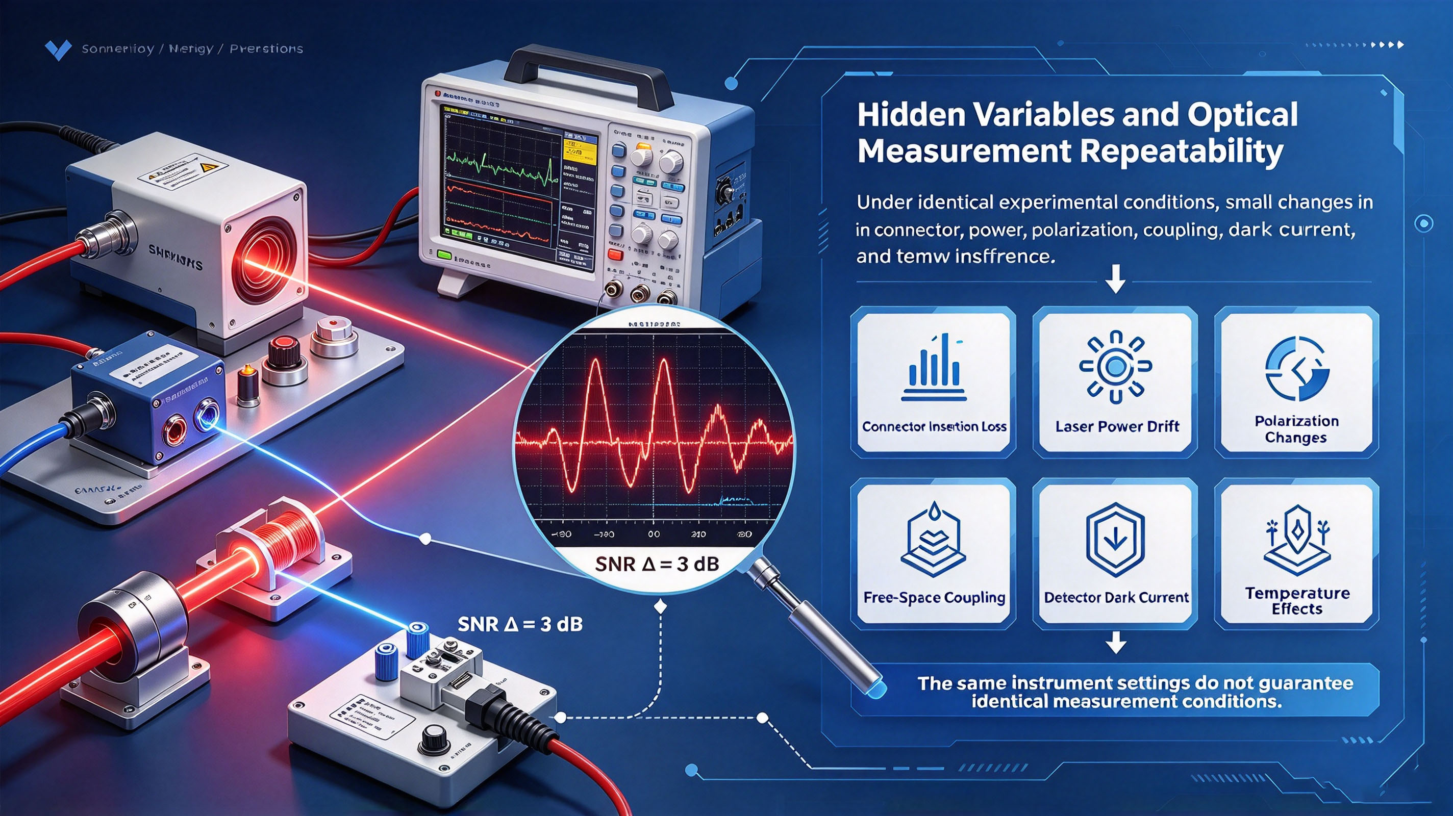
Why Does the Same Experiment Give an SNR Difference of 3 dB? Can Your Optical Experiment Really Be Repeated?

You run an optical experiment and get:

SNR = 32 dB

The result looks excellent.

The next day, you repeat the experiment using:

• the same fiber patch cord

• the same laser drive current

• the same photodetector

• the same measurement parameters

But this time:

SNR = 29 dB

A 3 dB difference.

You did not change any instrument settings.

The only things you did differently were reconnecting the fiber connector and realigning the optical coupling.

So what happened?

The uncomfortable answer is:

In optical experiments, “the same parameters” does not necessarily mean “the same physical conditions.”

A 3 dB variation in SNR can result from several small changes that are easy to overlook.

Connector insertion loss, source power drift, polarization state, coupling alignment, detector temperature, and instrument stability can all contribute.

Each effect may appear small when considered independently.

Together, however, they can easily produce a measurement difference of several decibels.

---

1. Fiber Connector Reconnection: Physical Contact Does Not Guarantee the Same Loss

An FC/PC fiber connector may have a specified repeatability of less than 0.2 dB under controlled laboratory conditions.

But real-world engineering environments are rarely as clean or stable as a connector manufacturer's test setup.

The original source notes that practical single-insertion loss variation can reach approximately 0.3–0.5 dB under engineering conditions.

Why?

Several factors can contribute.

Contamination on the Ferrule End Face

A fiber connector end face may look perfectly clean to the naked eye while still carrying microscopic particles.

The source notes that particles in the approximate 2–5 μm range can increase the effective gap between the fiber end faces and introduce additional insertion loss.

Even a tiny contamination particle can therefore change the optical coupling condition.

End-Face Damage

Repeated mating and unmating can gradually introduce scratches or other microscopic damage to the connector end face.

For angled connectors, repeated mechanical contact can also affect the condition of the angled end face.

Connector Alignment Repeatability

The ceramic ferrule and sleeve determine the relative alignment of the two fiber cores.

Small mechanical differences after reconnection can change the coupling condition.

The source cites approximately 0.5 μm degradation in alignment accuracy after 500 insertion cycles under the referenced conditions.

The important lesson is:

“The connector is fully inserted” does not mean “the optical interface is identical to yesterday.”

---

2. Laser Power Drift: Constant Drive Current Does Not Mean Constant Optical Power

Another common assumption is:

“The laser drive current is unchanged, so the optical power must also be unchanged.”

Not necessarily.

A laser's optical output depends on more than its drive current.

Temperature, device characteristics, aging, and operating conditions can all affect the output.

The source gives an example in which a DFB laser has a specified short-term power stability of approximately ±0.01 dB over 10 minutes, while an SNR experiment may run for two hours.

Over a much longer measurement period, even a small temperature change can modify laser operating conditions.

The source gives a representative example:

• ambient temperature drift: approximately 0.5°C

• threshold-current change: approximately 0.1 mA

• output-power drift: approximately 0.1–0.2 dB

For broadband SLED or ASE sources, temperature sensitivity can be even more significant.

The source notes that a two-hour temperature drift can produce approximately ±0.3 dB output-power variation under representative conditions.

Therefore, when comparing two SNR measurements, you should not record only:

Laser drive current

You should also monitor:

Actual optical output power

This is especially important when the two measurements are separated by tens of minutes or several hours.

---

3. SNR Depends on Both Signal Power and Noise Floor

Another easy mistake is to monitor only the signal.

SNR is fundamentally a ratio:

$$SNR=\frac{P_{signal}}{P_{noise}}$$

or, when expressed in decibels:

$$SNR_{dB} = 10\log_{10} \left( \frac{P_{signal}}{P_{noise}} \right)$$

Therefore, a change in SNR can come from either:

• a change in signal power

• a change in noise power

• or both

For example, if the optical source drifts by 0.3 dB while the noise floor remains approximately constant, the measured SNR can shift accordingly.

The source notes that when two measurements are separated by more than approximately 30 minutes, source-power drift can produce signal variations on the order of 0.2–0.5 dB, even when the noise floor remains relatively unchanged.

This leads to a useful measurement rule:

When comparing SNR, always record both the signal level and the noise floor.

A single SNR number is not enough to identify the cause of a change.

---

4. Polarization: The Variable You Cannot See

Polarization is one of the most easily overlooked variables in fiber-optic experiments.

A standard single-mode fiber is not the same as a polarization-maintaining fiber.

Environmental stress, temperature changes, bending, and mechanical movement can change the residual birefringence of the fiber.

As a result, the polarization state at the output can change over time.

The source describes how linear polarization can evolve into an elliptical state and how the output polarization changes with stress, temperature, and vibration.

Why does this matter?

Because many optical components have polarization-dependent loss (PDL).

If a downstream component has PDL, changing the polarization state changes the transmitted optical power.

For example:

Polarization state changes

↓

PDL response changes

↓

Detected signal power changes

↓

Measured SNR changes

The source uses 0.1 dB or greater PDL as an example of a level that can become relevant in this situation.

---

5. The Photodetector Can Also Be Polarization Sensitive

The polarization problem does not necessarily end at the optical component.

Photodetector responsivity can also have some polarization dependence.

The source notes that detector polarization dependence may typically be below approximately 0.05 dB, but can become larger under certain coupling conditions, such as oblique incidence.

Therefore, after reconnecting a fiber, you may unintentionally change:

Fiber polarization state

→ PDL

→ detector response

→ measured signal

without changing a single instrument parameter.

This is why the source identifies polarization changes after fiber reconnection as an important suspect when experimental repeatability is poor.

---

6. Free-Space Coupling: Micrometer Alignment Matters

Free-space optical coupling is another major source of repeatability problems.

For a single-mode fiber, the optical mode is extremely small.

The source gives an approximate mode-field diameter of:

$$MFD\approx10.4\ \mu m$$

for SMF-28.

It also gives an approximate coupling sensitivity of:

$$0.5\ dB/\mu m$$

for lateral displacement under the referenced conditions.

This means that even a very small alignment difference can matter.

Suppose the optical coupling stage has a repeatability error of:

$$0.5-2\ \mu m$$

Then the resulting coupling variation can be approximately:

$$0.25-1\ dB$$

under the source's representative sensitivity.

From an engineering perspective, this is not surprising.

The optical mode itself is only on the order of several micrometers across.

A mechanical positioning error that feels negligible to a human operator can therefore be very significant optically.

---

7. Thermal Expansion Can Move the Alignment Without Anyone Touching the Setup

Even if nobody touches the alignment stage, the coupling can still change.

Consider an aluminum optical mount.

Its linear thermal expansion coefficient is approximately:

$$23\ \mu m/(m\cdot^\circ C)$$

If the relevant mechanical distance is approximately 100 mm, then a 1°C temperature change produces an expansion of approximately:

$$23\ \mu m/m \times0.1m = 2.3\ \mu m$$

The source estimates that this can translate into approximately 0.5–1 dB of coupling variation under the referenced optical sensitivity.

This creates an important experimental insight:

A free-space optical setup can move optically even when it appears mechanically stationary.

The experimenter may return the next day and find that every stage is in exactly the same position, yet the optical coupling is different because the thermal state is different.

---

8. Detector Dark Current Also Changes with Temperature

The photodetector contributes another potential source of variation.

For an InGaAs PIN photodiode, dark current is strongly temperature dependent.

The source notes that dark current can approximately double for every 8–10°C increase in temperature under representative conditions.

Suppose the laboratory temperature changes from:

$$22^\circ C$$

to:

$$25^\circ C$$

between two measurements.

The dark current increases, which increases the associated shot-noise contribution.

The source estimates approximately:

• 30% increase in dark current

• approximately 14% increase in the corresponding shot-noise component

• approximately 0.5 dB SNR degradation under the stated conditions

This is another reason why recording laboratory temperature is not merely a formality.

For low-signal measurements, detector temperature can become part of the measurement uncertainty budget.

---

9. Six Variables Can Easily Become a 3 dB Difference

The source summarizes six potential contributors:

Variable	Representative variation
Connector loss	0.1–0.5 dB
Light-source power drift	0.2–0.5 dB
Polarization-state change	0.1–0.3 dB
Free-space coupling error	0.25–1 dB
Detector dark-current thermal drift	0.3–0.5 dB
Instrument instability	0.1–0.2 dB

The key point is not that these values should simply be added arithmetically.

Some variations are correlated, while others are independent or partially independent.

But the combined effect can readily reach the 2–3 dB range described in the source.

This explains why a 3 dB SNR difference does not necessarily indicate that one of the instruments is defective.

The experiment itself may simply not have been sufficiently controlled.

---

10. “Same Parameters” Does Not Mean “Same Experiment”

This is perhaps the most important lesson.

Suppose you record:

• laser current = 100 mA

• detector gain = 10×

• integration time = 1 s

• wavelength = 1550 nm

and reproduce exactly the same settings the next day.

The experiment is still not necessarily identical.

Other variables may have changed:

Fiber connection

→ different insertion loss

Polarization

→ different PDL interaction

Coupling

→ different mode overlap

Laser temperature

→ different optical power

Detector temperature

→ different noise floor

Environment

→ different thermal and mechanical conditions

Therefore:

Experimental repeatability is not the ability to reproduce instrument settings. It is the ability to reproduce the relevant physical conditions.

---

11. How to Improve SNR Measurement Repeatability

The good news is that most of these variables can be monitored or controlled.

Record the Environment

For every measurement, record at least:

• ambient temperature

• humidity if relevant

• connector insertion count

• laser warm-up time

• measurement start time

The source specifically recommends recording ambient temperature, connector insertion count, and source warm-up time.

---

Measure Optical Power Before and After the Experiment

Measure the source power immediately before and after the SNR measurement.

Also record detector dark current.

This makes it possible to determine whether the optical source or detector changed during the experiment.

A simple measurement log can therefore contain:

Parameter	Before	After
Laser power	—	—
Detector dark current	—	—
Ambient temperature	—	—
SNR	—	—

This simple procedure can eliminate a surprising amount of uncertainty.

---

12. Control Polarization in Polarization-Sensitive Experiments

If the experiment is sensitive to polarization, standard single-mode fiber may not provide sufficient repeatability.

Possible approaches include:

• use polarization-maintaining fiber

• minimize unnecessary fiber movement

• use a polarization controller

• characterize PDL of downstream components

• use a polarization scrambler where appropriate

The source specifically recommends using a polarization-maintaining fiber environment for polarization-sensitive experiments, or introducing a polarization scrambler before the PIN detector when appropriate.

The correct choice depends on what the experiment is intended to measure.

If polarization is part of the experimental variable, you should control it deliberately rather than allowing it to change randomly.

---

13. Don't Take One SNR Number Too Seriously

If your SNR measurement changes over time, do not immediately select the highest number.

Instead, perform a time-series measurement.

For example:

Continuous measurement

↓

30-minute or longer dataset

↓

Analyze stability

↓

Identify the stable region

↓

Calculate the representative SNR

The source recommends continuous measurement for approximately 30 minutes and using Allan variance to identify when the data become stable.

For repeated experiments, collect multiple datasets and report a statistical result rather than a single best value.

The source recommends using multiple repetitions and reporting the median ± standard deviation rather than relying on one measurement.

---

A Better Definition of Experimental Repeatability

A common definition of repeatability is:

“Run the same experiment again and get the same number.”

For optical experiments, that definition is incomplete.

A better approach is:

Step 1 — Identify the variables that influence the measurement

For SNR, these may include:

• optical power

• connector loss

• polarization

• coupling efficiency

• detector noise

• temperature

• instrument stability

Step 2 — Determine which variables can drift

Not every variable needs to be perfectly fixed.

Some can be monitored instead.

Step 3 — Control the important variables

Use:

• stable optical mounts

• controlled temperature

• proper connector cleaning

• stable fiber routing

• sufficient source warm-up

• polarization control

Step 4 — Quantify the remaining variation

Repeat the experiment multiple times and calculate statistical variation.

This produces a much more meaningful assessment of repeatability than comparing two isolated SNR numbers.

---

The Key Engineering Lesson

If you run the same optical experiment twice and obtain:

$$32\ dB$$

and:

$$29\ dB$$

do not immediately assume that something is wrong with the instrument.

A 3 dB difference can be the combined result of several small physical changes:

Connector

→ insertion-loss variation

Laser

→ output-power drift

Fiber

→ polarization-state change

Free-space coupling

→ micrometer-scale alignment error

Detector

→ temperature-dependent dark current

Environment

→ thermal and mechanical drift

The most important lesson is:

Optical experimental repeatability is not about keeping the instrument settings identical. It is about controlling or monitoring the physical variables that actually determine the measurement.

You do not necessarily need to eliminate every source of variation.

You need to understand which variables can move, determine how strongly they affect the result, and build them into the experimental procedure.

Because in precision optical measurements:

The number you get is only as repeatable as the physical conditions that produced it.